
Modeled after observed biology and behavior within the brain, neural networks are arguably the most popular of the biologically inspired AI methods. Neural networks excel at pattern recognition and classification tasks including facial, speech, and handwriting recognition. They also often play a central role in video game character AI.
Generally speaking, there are two types of neural networks: biological neural networks and artificial neural networks.
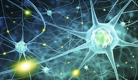
Biological neural networks are structures of interconnected neurons. Neurons, the primary cells of the nervous system, can be found in the brain, spinal cord, nerves, and other parts of the nervous system. While much is known about their composition, structure, and the functionality of the neurons themselves, scientists still know relatively little about how the neurons work together as a network in the brain to provide intelligence, learning, and memory.
Artificial neural networks (ANN), also called simulated neural networks (SNN), are mathematical and/or computational models that were originally developed to simulate, in a greatly simplified manner, biological neural networks. Artificial neural networks can be electrical, mechanical, computer programs, or a combination of all three. In robotics, computer science, and related fields, the word “artificial” is usually dropped from the term. When one speaks of neural networks it is generally assumed that they mean artificial neural networks.
Biological Neural Networks
The human brain is composed of a network of billions of tiny cells called neurons that communicate with one another through electrochemical impulses. Estimates differ, but most scientists suggest the number of neurons in the human brain to be in the neighborhood of 100 billion (1011).

Structure of a Typical Neuron
Although there are many types of specialized neurons that vary greatly in appearance, they all consist of three main parts:
- Soma – the cell body. It is the large central portion of the cell that contains the nucleus. It is between the dendrites and axon.
- Axon – a slender projection that carries nerve impulses away from the neuron. The lengths of axons vary from neuron to neuron, but some may be several orders of magnitude longer than the diameter of the soma itself. Each neuron only has a single axon, but that axon may have multiple branches. These axon terminals are able to communicate with multiple target neurons.
- Dendrites – short, tree-like cellular extensions from the soma. They receive electrical stimulation from other neurons.
Neurons communicate with one another through specialized connections called synapses. A synapse is formed when the axon terminal of one neuron, known as the pre-synaptic neuron, couples with the dendrite or soma of a second neuron, the post-synaptic neuron. This is not a physical connection. Rather, the membranes of the axon and dendrite face each other across a very narrow gap. The arrival of the neural impulse, also called the action potential, at the axon terminal of the pre-synaptic neuron triggers the release of a chemical neurotransmitter. This neurotransmitter passes rapidly by diffusion across the synaptic cleft to the dendrite of the post-synaptic neuron. The neurotransmitter arriving at the post-synaptic neuron will influence it in one of two ways: it will stimulate it, or it will suppress (inhibit) it. This neuron will itself fire, sending its action potential out its own axon, but only if and when the sum of all of its incoming potentials reach a threshold value known as its threshold potential. The number of other neurons a neuron connects to varies widely, but can be anywhere from ten to several thousand. Scientists estimate that there are 100 trillion (1014) synapses (neuron to neuron connections) in the human brain.
The change in the potential across the post-synaptic membrane during activation of the synapse, the post-synaptic potential, defines the “strength” of the synapse. Stronger synapses exhibit larger changes. Additionally, potential changes can fall into one of two categories: short term with no changes to the neurons, or long term and excitatory (long term potentiation – LTP) or long term and inhibitory (long term depression – LTD). During LTP or LTD repeated or continuous stimulation causes a physical change in the post-synaptic neuron itself. For example, the post-synaptic neuron may create new receptors in its dendrites for receiving neurotransmitters or the efficacy of its receptors may be increased by a process called phosphorylation, thereby “strengthening” the synapse. As a post-synaptic neuron integrates it’s incoming signals and compares that sum to it’s threshold potential to determine if it should fire, stronger synapses will contribute more to that sum (or decrease more in the case of suppression) than weaker synapses. Changes to the response characteristics of synapses are known as synaptic plasticity, and it is believed to be the key to memory and learning. This will be more clearly illustrated in our discussion of artificial neural networks.
This is a grossly oversimplified overview of biological neurons and synapses. However, it should be more than sufficient background for understanding the algorithms behind artificial neural network models and simulations.
Artificial Neural Networks
Like the biological networks they are modeled after, artificial neural networks are collections of basic computational units called nodes, interconnected in a parallel fashion. Unlike the brain, artificial neural networks have far fewer nodes than a brain has neurons, and the nodes are far simpler in their functionality than the neurons they represent. This, however, does not stop artificial neural networks from exhibiting characteristics associated with the brain including learning and memory, albeit on a much more limited scale.
The basic unit of the artificial neural network is the node. This corresponds to a neuron in a biological neural network. Each node has series of inputs analogous to the synapses formed at the dendrites of a post-synaptic neuron. And like the synapses of a post-synaptic neuron, each of these inputs to a node has a “weight” associated with it. A node will also have one or more outputs which correlate to the synapses formed by axon terminals of the neuron’s axon connecting to dendrites of other neurons.
A node has an activation function, also called a transfer function, which like the threshold potential of a biological neuron, tells a node when to fire. The sum of the weights of each input multiplied by their respective values are fed into the transfer function, and the resulting value is the node’s output. The simplest transfer function is a binary step, or transfer, function yielding a discreet value if the summed inputs are greater than a set threshold value, or a smaller discreet value otherwise. Often 1 and 0 are used to represent firing and not-firing states respectively, but other values like 1 and -1 are used as well.
The step function is suitable for only very basic applications. In most networks many, if not all, of the nodes have a more complex function. A sigmoid curve is often chosen for the transfer function. It introduces non-linearity into the performance of the network while still “squashing” the activation of node into the range of [0,1]. The tanh function is often used as well since it behaves similarly although its activation range is [-1,1].
The simplest and one of the more common artificial neural networks is a feed-forward neural network. In this type of network, the nodes are arranged in layers. A node in one layer is connected to every node in the next layer. There are usually three layers: an input layer, a hidden layer, and the output layer. The input layer’s sole purpose is to accept the data array supplied to the network. Processing is done in the hidden and output layers. The activation of the output nodes represents the answer or solution to the calculation.
In order for a neural network to yield meaningful results it must be trained. Initially the weights of the connections between all of the nodes in the network are set to random values. When data is presented to the input layer, the nodes will fire randomly based on their input values, input weights and transfer functions, and the output will be random as well. In this state the network has no knowledge. During training, a series of data with known output values is fed to the network. After the output is obtained for an input the connection weights are adjusted based on a learning algorithm in an effort to match the desired, or correct, output. Ideally after training the known data should produce the correct, predicted results, but more importantly the network can now be fed unknown data, and the network should yield output that is meaningful and correct.
The functionality of neural networks makes them ideally suited for classification and identification tasks. For example, pictures of dogs and pictures of cats can be used to train a network. Regardless of the breed or any other characteristic of the dog, the correct output of the network is a combination of output nodes firing to designate the classification ‘Dog’, and the same is true for cats. Once trained, you should be able to feed the network a picture of a dog, and although it may not be a breed, or a color, or sex, or size, etc. that was used to train the network, the network should still output ‘Dog.’ A trained network therefore has knowledge. In this case it knows what a dog looks like.
This concludes my overview of neural networks. By knowing the basic structure and functionality of biological neural networks, one can more easily understand how to model and build artificial neural networks for a host of purposes. This article did not delve into any algorithms, math or computer code associated with neural networks, but several articles that should be published in the near future will.