
This is the second article in the series about artificial neural networks. If you have not already done so, I recommend you read the first article, “Neural Networks: The Node“, before proceeding. It covers material that should be understood before attempting to tackle the topics presented here and in future articles in this series.
There are several properties that define the structure and functionality of neural networks: the network architecture, the learning paradigm, the learning rule, and the learning algorithm.
Network Architecture
Artificial neural networks consist of one or more layers of nodes. The organization of the connections between these nodes falls into one of two categories: feed-forward or recurrent.
Feed-Forward Networks
In feed-forward networks the nodes are organized so that the output of a node in one layer connects to the input of every node in the layer above. The signal flows in one direction: from lower layers to intermediate layers and ultimately to the output layer. There is no signal flow from higher to lower layers and no connections between nodes in the same layer.
Frank Rosenblatt invented the perceptron, the first feed-forward neural network, in 1957 at the Cornell Aeronautical Laboratory. Expanding on McCulloch and Pitts’ work, Rosenblatt’s initial perceptron was a single layer of MP neurons that processed an array of inputs and were activated (or not) based on their threshold values.
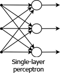
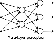
It is important to note that many people would call this a 2-layer network. Others do not count the input layer as a true layer and only count the layers that have nodes with weighted inputs as actual layers. A single MP neuron, as illustrated in “Neural Networks: The Node,” can perform classifications. It is also, therefore, the simplest perceptron. MP neurons are actually often referred to as perceptrons in literature. Initially there was very much excitement about single layer perceptrons and their ability to classify, although this was soon dampened by the discovery that they could only learn linearly separable patterns (to be discussed in a coming article). This limitation was eventually overcome by the use of “hidden” layers in a multi-layer perceptron.
Recurrent Layer (Feedback) Networks
In recurrent layer networks, also known as feedback networks, the nodes in a layer may have connections to other nodes in the same layer, and may also have incoming, feedback connections from higher layers in addition to their output connections to the higher layer. There are many types of recurrent networks including Competitive, Hopfield, and Kohonen’s SOM.
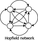
The type of architecture will affect the network behavior. Feed-forward networks are static and memory-less. Only one set of output values is produced from an input, and the response to the input is not affected by the previous network state. Feedback systems, on the other hand, are dynamic. When a new input is fed to the network, the outputs are calculated. Then by means of the feedback connections the weights of the entire network are recalculated, and the outputs are modified based on this new network state.
Learning
The process of learning by neural networks involves modifying the network architecture and updating the connection weights of the network so that it is able to satisfactorily perform a given job. Usually training sets are fed in, and the weights are adjusted as the network learns the underlying rules of the example sets. ANN’s therefore learn by example. They do not have a set of rigid rules programmed into them but are instead able to extract the input-output relationships from the training data. They can often find nuanced rules and relationships between data that humans may not be able to easily recognize, making them more flexible and powerful than traditional expert systems.
Network learning is broken down into three interrelated properties: the learning paradigm, the leaning rules, and the learning algorithm. The learning paradigm is dictated by the data that is available to the network for training and regular operation. The learning rules describe exactly how network weights are updated, and the learning algorithm is the actual procedure outlining how and when the learning rules are applied.
Learning Paradigms
There are three learning paradigms: supervised, unsupervised, and hybrid.
Supervised Learning
During supervised learning a series of input patterns are fed into the network. For each input pattern there also exists a desired, or correct, output pattern. After each input is evaluated, the actual output is compared to the desired output and the weights are adjusted in attempt to match the two. This is also known as learning with a “teacher.” Reinforcement learning is a type of supervised learning where the network is informed of incorrect output during training but not provided with the correct answer. Weights are adjusted based on its learning algorithm.
Unsupervised Learning
Unsupervised learning does not make use of correct answers during training. The network is only provided with the training inputs, and it uses it’s learning algorithm to discover patterns and relationships in the training data. Its weights are adjusted during training to reflect the categorization of the data it has been presented.
Hybrid Learning
Hybrid learning is a combination of the other two paradigms. Supervised learning is used to train some of the weights while unsupervised learning is used to train the rest.
Learning Rules
There are three factors that will dictate the type of architecture, learning rules and algorithm used: network capacity, sample complexity and computational complexity.
The capacity of an artificial neural network is how many different patterns it can store, as well as how it is able to form decision boundaries between them.
Sample complexity refers to the number of training samples that are needed to fully train the network. Using too few patterns will cause a situation known as “over fitting” where the network is trained to identify only those patterns used for training, but not able to recognize other patterns similar to, but not exactly the same as, the training samples.
The computational complexity is the amount of time it takes for an algorithm to finish learning during training. Most algorithms are complex and computationally intensive, requiring a relatively long period of time to complete. Finding an optimal balance between computational complexity and network effectiveness is the goal of many neural network researchers.
There are four basic types of learning rules: error-correction, Boltzman, Hebbian, and competitive learning. Because of the intricacies and mathematics involved with the different rule types and their associated algorithms, I will be dedicating separate articles to each of them starting with error-correction. Please check back again soon as I intend to publish it in the very near future.